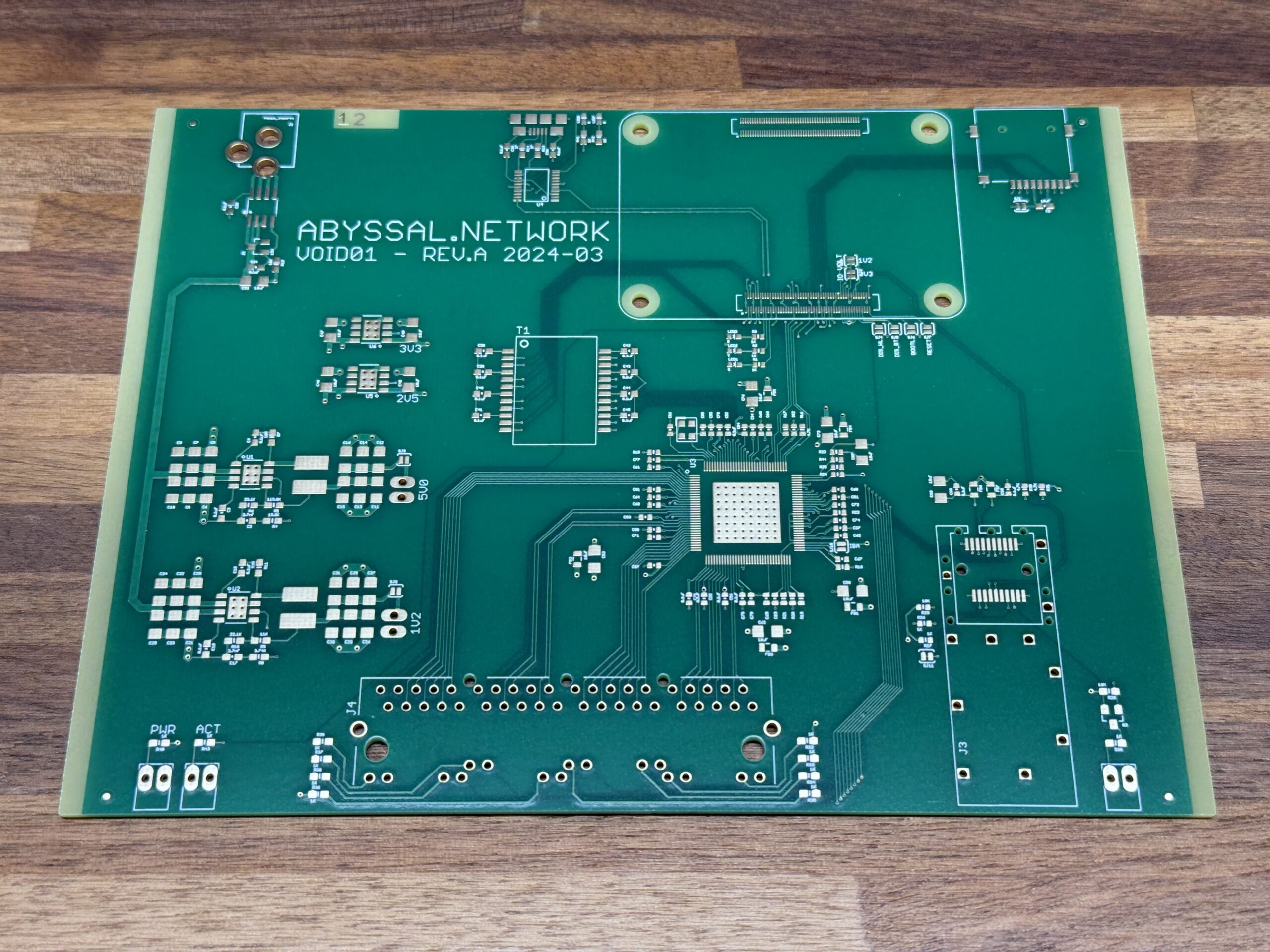
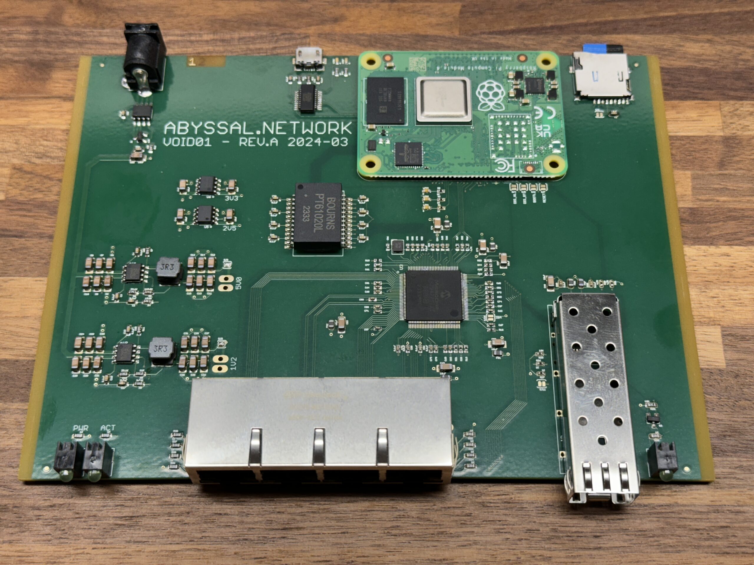
Wired Ethernet on ESP32

I’ve used the ESP32 microcontrollers for a number of projects at this point, often using the built-in WiFi radio. However, there are use cases where WiFi may be less than ideal. In my case, I’m interested in the higher reliability a wired connection offers, as well as consistent latency performance.

Fortunately, the ESP32 includes a built-in Ethernet MAC, which is the controller that manages a wired Ethernet connection. If we can pair that with a PHY, which drives the actual electrical signals on the wire, we should be able to get a working connection.

Before getting into a specific project, I wanted to put together a test board to feel out how it would work, and resolve any issues before putting it to real use. Fortunately, there’s a few references around, including a very nice open source design from Olimex that proved to be a useful reference combined with the part datasheets.

I didn’t bother to include Power over Ethernet like their design does, though that is another potential benefit over WiFi, where you can have a single cable provide power and data to a project.

I ended up testing my design by coding up a simple NTP server, and feeding the board from a GPS signal. I started with MicroPython, which is quite handy for putting together an application a lot faster than writing it in C++, but ran into performance issues that negatively impacted the quality of the time responses the board was able to return.

After rewriting in C++, the board returns fairly accurate timing responses, and would be an interesting basis for future work, though isn’t really in a state suitable for publishing currently.

Posted in Electronics, Technology | Leave a comment

GPSMON Output with UBlox Receivers

I’ve got a UBlox GPS module in a somewhat challenging RF environment (Indoor with no clear sky view, and potentially some other RF sources causing interference), and have been looking at what data I can gather with regards to the signal. The receiver is attached to a computer running GPSd, so the easiest first step it to look at what data we see in the ‘gpsmon’ utility.

Some fairly self explanatory stuff here, receiver channel, satellite ID, azimuth, elevation, signal to noise ratio, and whether that satellite is being used in the fix. However, that flag field is not entirely clear, and some google searches didn’t bring it up either. I wasn’t able to find any documentation on what that flag field represented.

We can, however, reference the UBlox datasheet and look at the UBX-NAV-SVINFO message, which is the message that contains all this info on the individual satellites being tracked, and that gpsd / gpsmon is parsing out for us.

There end up being two bytes output for each satellite, that are labelled as ‘quality’ and ‘flags’ in the datasheet, and manually parsing the raw data, I was able to confirm that gpsmon is showing us here these two bytes in hexadecimal. The first byte being the ‘quality’ byte, and the second one being ‘flags’.

To use the example of PRN 21, on channel 5, gpsmon is showing us the data ‘070D’. Now we just need to cross-reference this with the datasheet.

The first byte we got is ’07’ hexadecimal, which is 7 decimal, and that matches the “Code and carrier locked and time synchronized” state in the quality table. All good there.

The second byte we got is ‘0D’, which is 00001101 in binary, and so we see that matches with the svUsed, orbitAvail, and orbitEph bits. So this satellite is being used in the fix, and we have current orbit information and ephemeris for this satellite.

So now we now how to parse out the flags information gpsmon will provide to us for UBlox modules, and better debug the state of how the receiver is tracking the constellation.

Posted in Electronics, Random | Leave a comment

Simulating Full IPv4 Tables in the Lab

I’ve been doing some testing recently with different software based routers, and wanted to give them a test under real world conditions. The current full IPv4 table is larger than 900,000 routes and to get an idea of how well they handle it, I needed to be able to simulate getting a full transit feed in the lab environment.

This is far from a new topic, and I’m sure there’s many ways to approach this issue, I just happened to need to work on this recently, and this is the method I ended up settling on.

First, we need a source for all these routes. They don’t necessarily have to be real, we could just make fake routes for 1.1.1.1/32, 1.1.1.2/32, 1.1.1.3/32, and so on till we got to 900,000(ish) total, but in some cases this can be an unrealistic test as systems will merge routes into contiguous blocks of larger prefixes and internally reduce the size of the routing table. To replicate how reductions would happen in the real world, we need the real world routes.

Fortunately, RIPE maintains a number of servers that regularly save a copy of all the routes received, from a variety of locations around the world, and provide that for download. I looked at their list of servers, and selected RRC18 as it has a single full table, which matches what I’m aiming to emulate. You could of course select another server that gets multiple copies of the full table from different peers if that data better fits your test environment. Then you just download the latest dump from your selected server, in my case: https://data.ris.ripe.net/rrc18/latest-bview.gz

I originally thought the easiest use of the data might be to use some bash and awk one-liner to parse the output of the file with bgpdump, and generate a text file with commands to add them as static routes to a VyOS instance, and I’d BGP peer that to the test lab. However, loading the routes to VyOS choked on the massive quantity. The first route addition commands went quickly, eventually slowing to a crawl as ever more routes were added. Eventually I gave up after leaving it trying to process the static route creations for several hours.

I tried tweaking my bash and awk to output a config file for FRR under linux that contained all the static routes, but FRR choked, using more than 64GB of memory and being killed when the system ran out of RAM.

An acquaintance pointed me to gobgpd, which will work on the dump from RIPE directly, and is a very simple daemon to test with BGP. Turns out it works pretty well.

You’ll want to:

  • install via your distro’s package manager of choice, “apt-get install gobgpd” or equivalent.
  • Create gobgpd.conf (example below)
  • Start gobgpd with “sudo -E gobgpd -f gobgpd.conf &”
  • Load the route dump into the daemon with “gobgp mrt inject global latest-bview”

Here’s a very quick config example for you. This config should be pretty self documenting in terms of the local AS and router-id, and the neighbor configuration. The policy is there to overwrite the next-hop data from the dump, as their next-hop data obviously won’t work for us here.

[global.config]
  as = 65500
  router-id = "192.168.1.1"
[[neighbors]]
  [neighbors.config]
    neighbor-address = "192.168.1.2"
    peer-as = 65501
[[policy-definitions]]
  name = "policy1"
  [[policy-definitions.statements]]
    name = "statement1"
    [policy-definitions.statements.actions.bgp-actions]
      set-next-hop = "192.168.1.1"
[global.apply-policy.config]
  export-policy-list = ["policy1"]
  default-import-policy = "accept-route"
  default-export-policy = "accept-route"

And once it’s running, we can check on the BGP state on our peer, in this case a VyOS test VM.

nigel@vyos01:~$ show bgp summary

IPv4 Unicast Summary (VRF default):
BGP router identifier 192.168.1.2, local AS number 65501 vrf-id 0
BGP table version 916895
RIB entries 1679949, using 308 MiB of memory
Peers 1, using 725 KiB of memory

Neighbor        V         AS   MsgRcvd   MsgSent   TblVer  InQ OutQ  Up/Down State/PfxRcd   PfxSnt Desc
192.168.1.1    4      65500    945727     15503        0    0    0 00:05:24       916835        0 N/A

Total number of neighbors 1

Now we’ve got a full table of 916,835 routes, with real data, in our lab environment for testing.

Posted in Random, Technology | Leave a comment

GPS Timing Over USB

I recently posted about building this GPS receiver for use in making Stratum 1 NTP servers, and through conversation with some friends, I was interested understanding the performance difference in timing the Pulse-Per-Second (PPS) signal via the hardware serial port, and via the USB port.

In this discussion we are looking at the timing of the DCD pin change which the PPS signal is connected to. Most USB based GPS receivers do not expose the PPS signal via the DCD line, which is part of why I built mine. My receiver uses the FTDI FT231XS chip for handling the USB serial port, and supports the DCD line (along with a number of others). There are a number of folks I’ve seen write tutorials which base timing off of the arrival of the NMEA text strings the GPS puts out, which is entirely unsuitable. The output of NMEA strings is not a strictly controlled timing source from the GPS, and should *ONLY* be used for coarse time setting. We’ll also see below that there are additional error sources impacting the accuracy of timing on the string data as compared to the DCD line.

There has been a long-touted statement that USB is unsuitable for capturing the precise timing of the PPS signal from a time source like a GPS due to USB being a polled bus. The end device can’t initiate an interrupt, and has to wait for the host computer to get around to asking it for data. A hardware serial port on the other hand has the capability to have interrupts trigger on things like the DCD line changing state, and thus the system can quickly capture the timing of the event.

On the surface these two things make sense, but I became interested in *how much* worse the USB device would perform. Not every host system has an available serial port, and USB might prove to be pretty reasonable, even if not as good.

I began the investigation by installing a clean Ubuntu 22.04 LTS image on a HP T620 thin client, and attaching the GPS to the hardware serial port. I configured gpsd and chrony per the docs in my github repo, and started logging the chrony tracking data.

Here on the hardware serial port, the system tracks GPS well, and the RMS (A kind of average) Offsets were generally pretty good with values on the order of less than 20uS (microSeconds).

After gathering that data, I used the same GPS device, but plugged it into the USB port instead to compare.

Here we see that when timing the signal via USB, the offsets are at best an order of magnitude worse, jumping pretty chaotically between 250uS and 350uS. This is definitely not as good as the hardware serial port by a long shot, but it’s still down around a third of a millisecond, and plenty good enough for most applications.

However, there’s a number of USB ports on this system, there’s even USB3 ports on it. The device (the FT231XS) is still only a USB2 device, so I should expect the same results… right?

What? Somehow the same USB2 device, when plugged into a USB3 port, is managing better timing than the hardware serial port. Not by a lot, but it is better. How does this work when USB is supposed to be always worse due to the polled nature of the bus?

I needed to get a clearer picture of how the FT231XS was interacting with the host. In my network engineering day job, we use TCPdump all the time to capture network packets for analysis. I figured there had to be some utility to capture data from the USB system. Turns out that utility is still TCPdump!

With the ‘usbmon’ kernel module loaded, TCPdump will actually capture packets from the USB system, and the Wireshark analysis utility will even parse them! I made a pair of captures, one from one of the poorly performing USB2 ports, and one from the magical USB3 port.

Here we see the USB2 capture on the left, and the USB3 one on the right. In the top portion of the window, I’ve highlighted the frame where the DCD line goes low and the FT231XS is reporting that data, and in the middle-ish portion of the window I’ve highlighted the time the computer thinks this frame has arrived.

You can see in the Epoch Time / Arrival Time lines, that on USB2, the system thinks this packet arrived 277uS after the second ticked over, and on USB3, the system thinks it arrived 2uS after the second ticked over. Let’s look at the overall set of frames to see how the FT231XS is behaving. Maybe it’s different when plugged into USB3 somehow?

Nope. The FTDI chip is behaving exactly the same way on each bus, which makes sense. The device itself only does USB2. It’s going to keep doing what it does. We also see an interesting pattern in the frames. The host is asking the device to report data, and the device is taking just under 16mS (milliSeconds) to reply, and then the host immediately asks again for more data. Repeat the cycle.

Except when the DCD line changes. In the frame where the DCD line changed, the FTDI chip didn’t take 16mS to reply, it replied much sooner. Clearly the chip is treating this differently somehow. Let’s look at what the chip asked for in the configuration info during initialization.

Here we see the configuration endpoints for reading data from the chip, and writing data out to the chip. It’s saying that the max packet size will be be 64 bytes, and it wants the polling interval to be 0. The FTDI folks are being clever here. For slower devices like a GPS, the NMEA data isn’t going to fill up the 64 byte buffer very fast, but they want to have the option to deal with things like the DCD line quickly, so the chip tells the computer to immediately poll again, but the chip will wait a little while (the 16 milliseconds we saw above) to let the buffer fill a little and make efficient use of the USB frame, *EXCEPT* if there’s a DCD change and all it has to do is stop waiting and respond immediately.

So, we’ve determined that the chip is acting the same way on both the USB2, and USB3 ports, and that the designers of the chip have taken considerations to make line changes report quickly. Why are the results so different then?

MAGIC. Well, chipsets, but effectively magic. The processor in a computer isn’t directly connected to the USB ports (or really most of the ports). The processor talks to the chipset (part of the motherboard) that handles a buttload of stuff, often including the USB ports. This gets into pretty opaque territory for me, and maybe someone with a ton of experience with chipsets / chipset drivers and config might be able to illuminate more, but it seems that ultimately the designers of this chipset decided that this performance was good enough for USB2, and that USB3 (as a newer & faster version) needed more.

However, that begs a new question. Will different chipsets treat this differently? Absolutely.

I got another system together, again with a fresh install of Ubuntu 22.04 LTS, but this time the system was server hardware rather than a little thin client. A SuperMicro box, with a Xeon CPU is surely a very different beast than the HP T620. Let’s compare the hardware serial port now to USB2.

Here we see the first part of the graph as the performance on the hardware serial port, the spike around 2:30PM is when I reconfigured it to use USB, and the latter part of the graph is performance on USB2. We see that the USB visually is very slightly worse, but is effectively comparable to the hardware serial port. In the case of this server hardware, with the chipset it was built with, the USB option seems to be just as good.

Circling back all the way to the beginning, does the saying that USB PPS signals aren’t as accurate as ones captured via a hardware serial port remain valid? It depends.

Clearly on some systems performance does suffer. On other systems, or even potentially different ports on the same system, you could see performance that meets or potentially marginally exceeds the hardware serial port. The only way to know is to measure it.

Of course, you still need a GPS with PPS signal, being fed into a quality USB adapter with proper handling for line changes. However, I’ve come out of this a lot more willing to think of USB as a viable option (with verification).

As a caveat, these tests were done with otherwise idle systems, and no other USB devices plugged in. Busier systems, or ones with other USB devices contending for time on the bus may impact performance in ways we haven’t seen in the testing above, but that’s science for the future.

Posted in Electronics, Projects, Technology | Leave a comment

Air Quality Sensor

A couple years ago I cobbled together a couple of air quality sensors to give my family and I a better idea of the state of the air in and outside our home, particularly during what seems to be becoming the annual fire season in the Pacific Northwest.

These were cobbled together devices mostly with parts I already had laying around, which worked fine, and continue to operate well, but as we approach another summer I was interested in putting together a couple additional sensors as well as improving the state of the hardware.

The sensor I’ve put together is based around an ESP32 reading data from a pair of Plantower PMS7003 particulate sensors, and a Bosch Sensortec BME280 Temperature, Pressure, and Humidity sensor. The data from all the sensors is then sent to my logging/graphing system via WiFi.

I took inspiration from the commercially available sensors from PurpleAir and designed it to fit within a 3″ PVC pipe cap, along with a 3D printed carrier, which provides for a nice outdoor enclosure that can be easily mounted in a variety of locations.

The 3D printed carrier has vent openings for the particulate sensors, and the temperature sensor extends below the main body to have the best exposure to the ambient temperature with minimized effects of internal heating, but still being sheltered under the cap.

I’m looking forward to getting a few of these deployed, and getting a better picture of the air quality in my area over the coming months.

Lastly, the project is open source and you can find all the resources on my GitHub repo.

Posted in Electronics, Projects, Weather | Leave a comment