
A quick photo of some holiday ornaments I made this year. The boards use RGB LEDs, silkscreen, and gold plating for decoration. The batteries will run it for more than 100 hours of continuous runtime. Made for some good little gifts for the family.
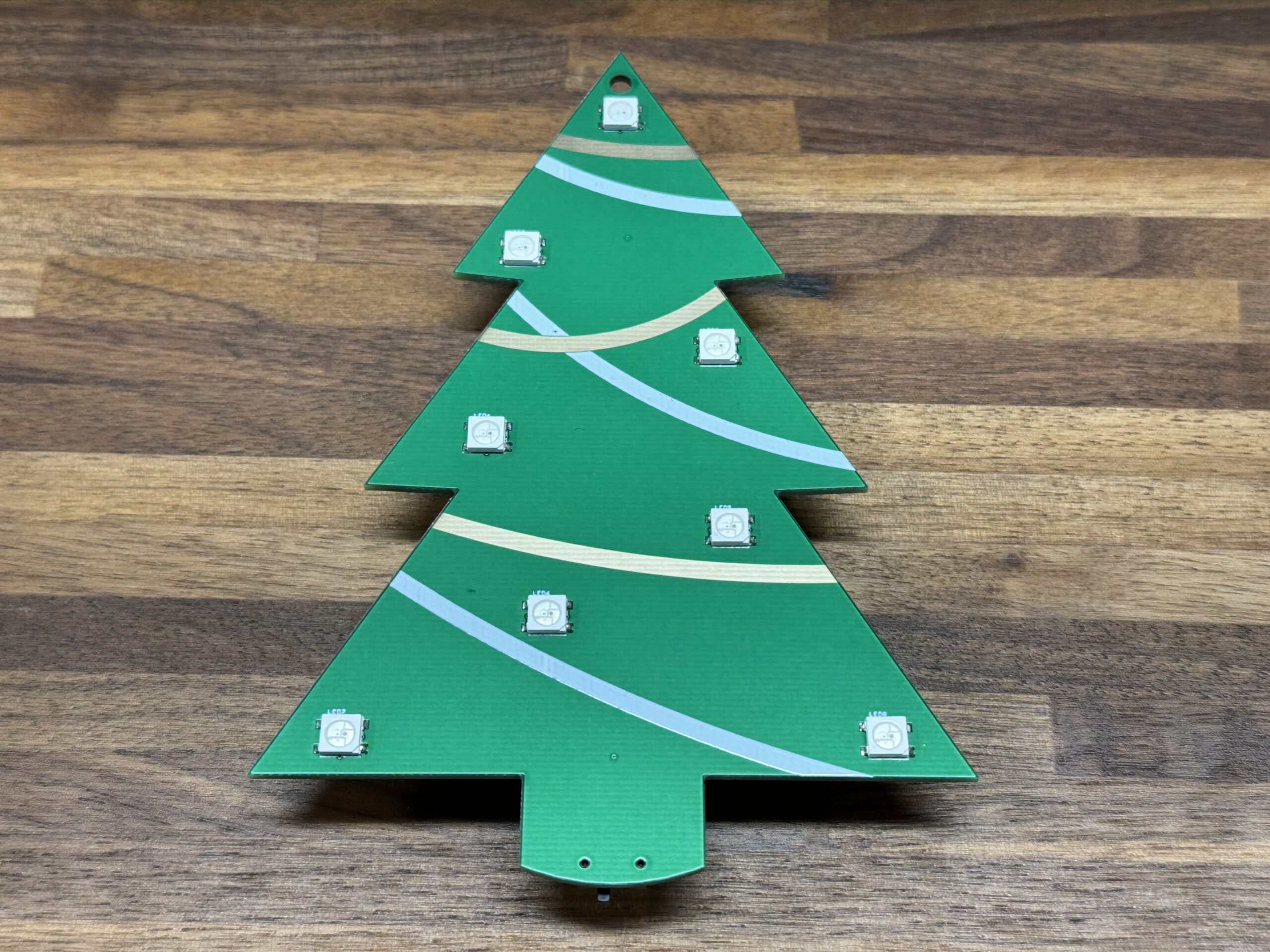
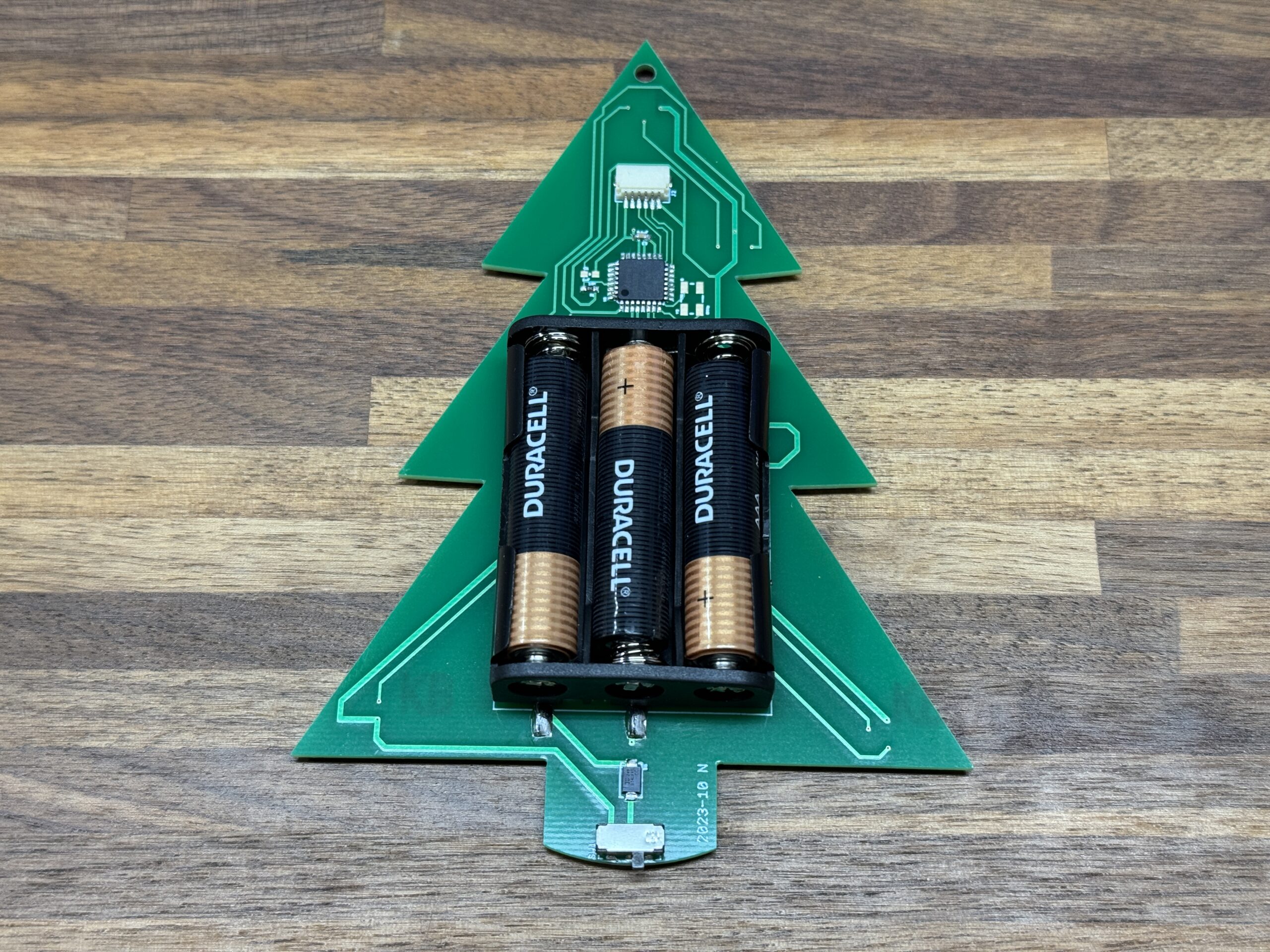
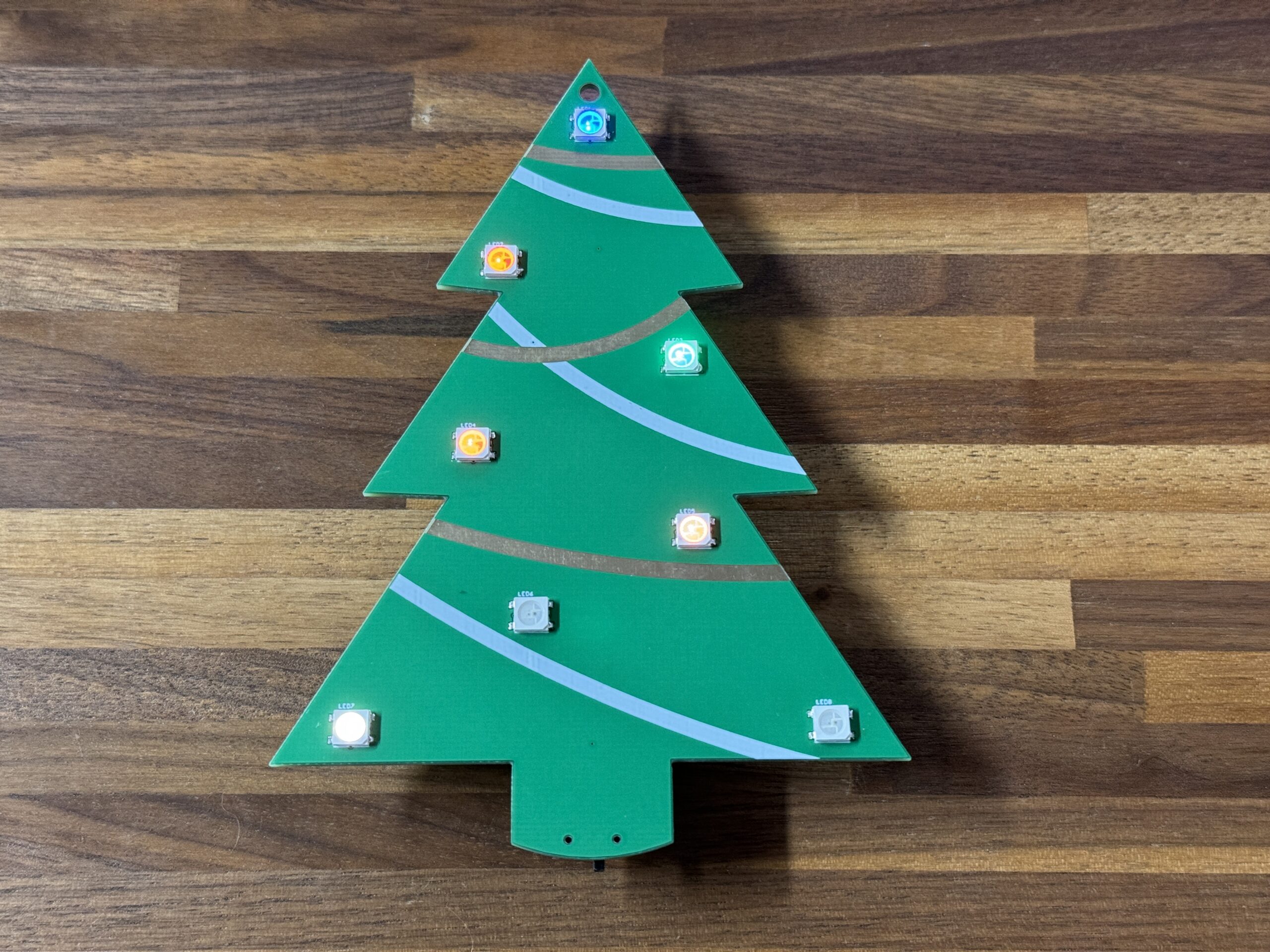
A quick photo of some holiday ornaments I made this year. The boards use RGB LEDs, silkscreen, and gold plating for decoration. The batteries will run it for more than 100 hours of continuous runtime. Made for some good little gifts for the family.
A little while back I was given one of my great grandmother’s mechanical clocks, which appears to be a Seth Thomas from (as best as I can tell) 1906. I remember this clock sitting on the mantle as a kid, but it’s been years since anyone in the family has had this in use, and was in desperate need of a cleaning / oiling.
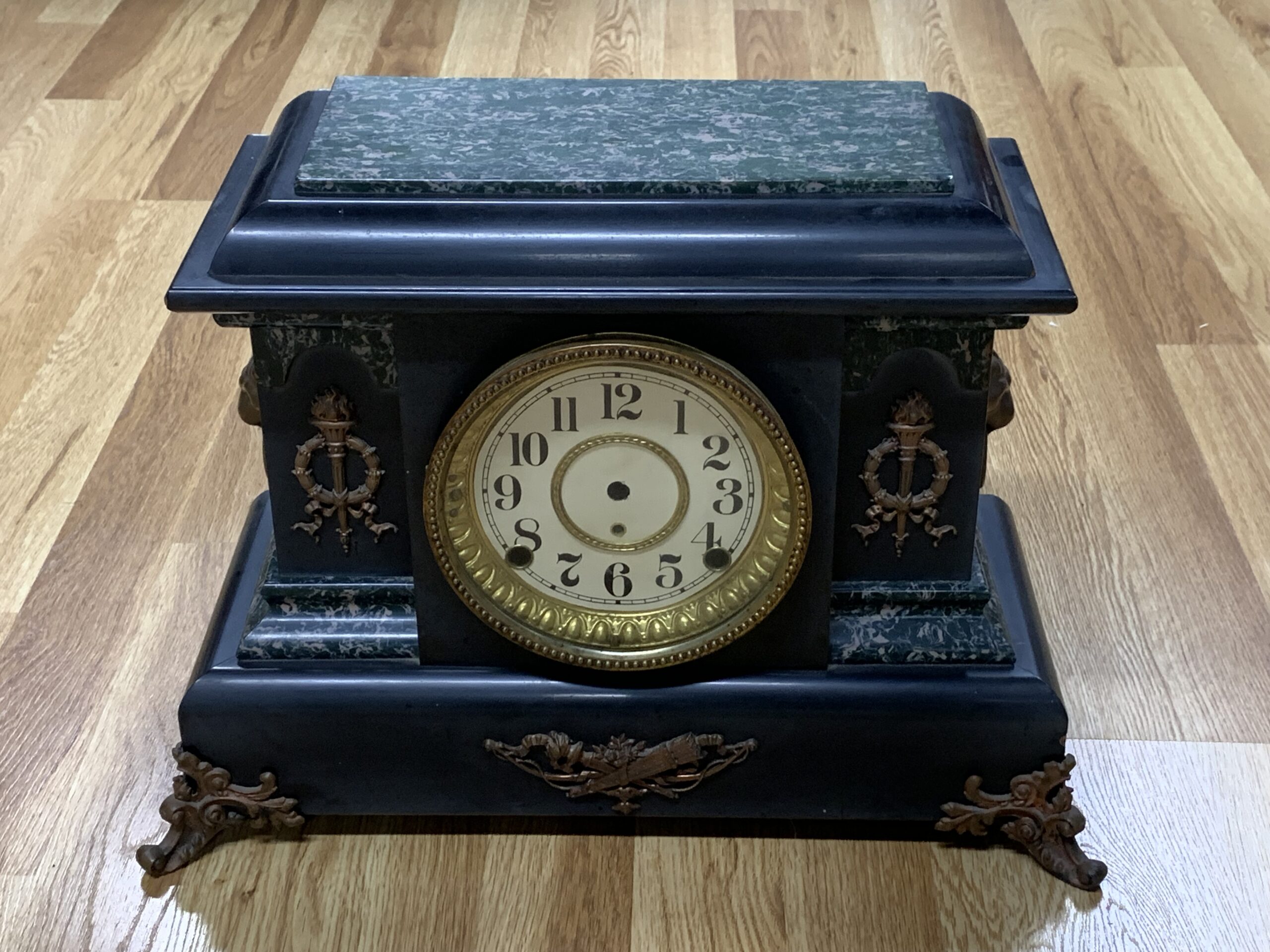
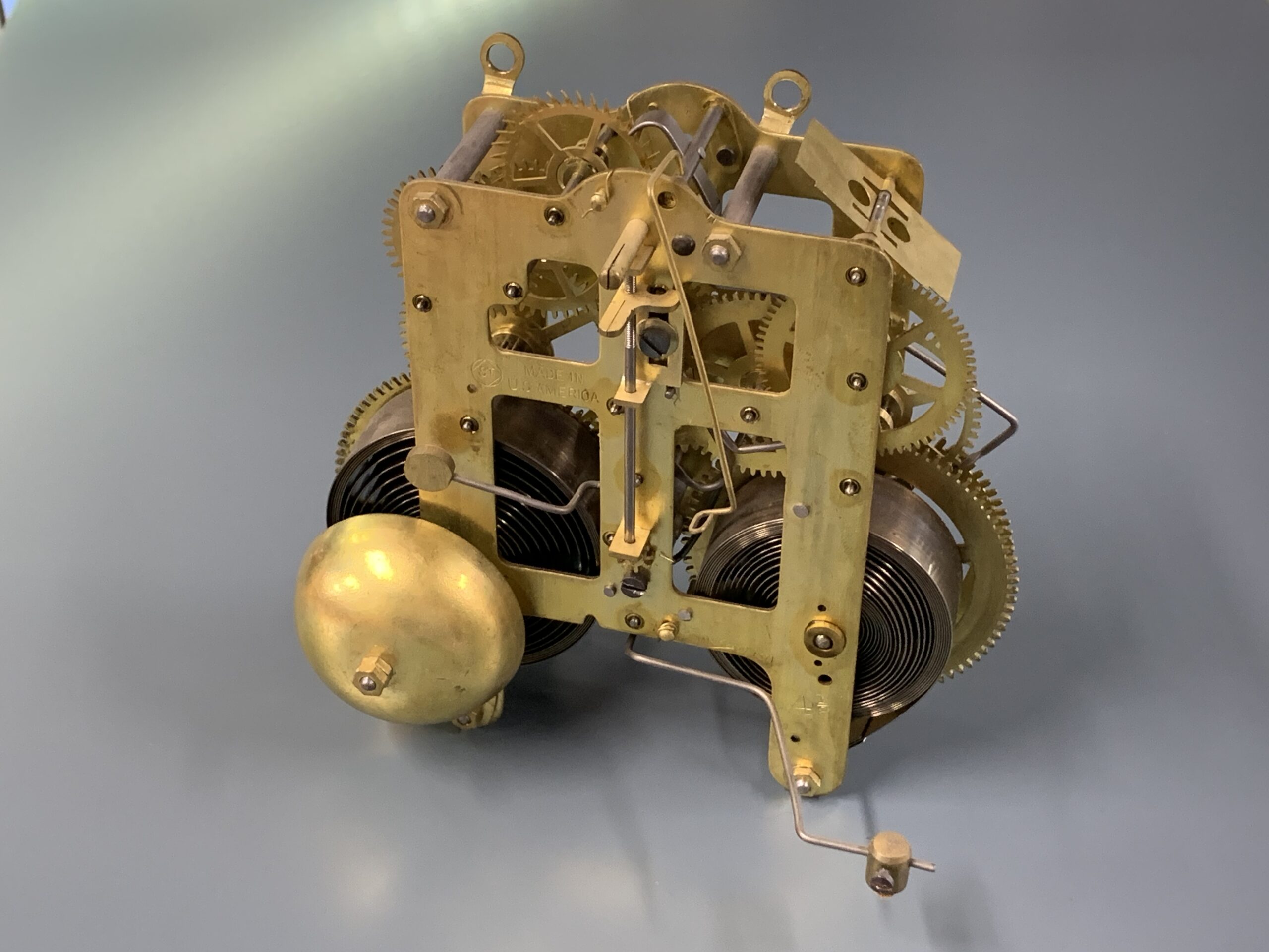
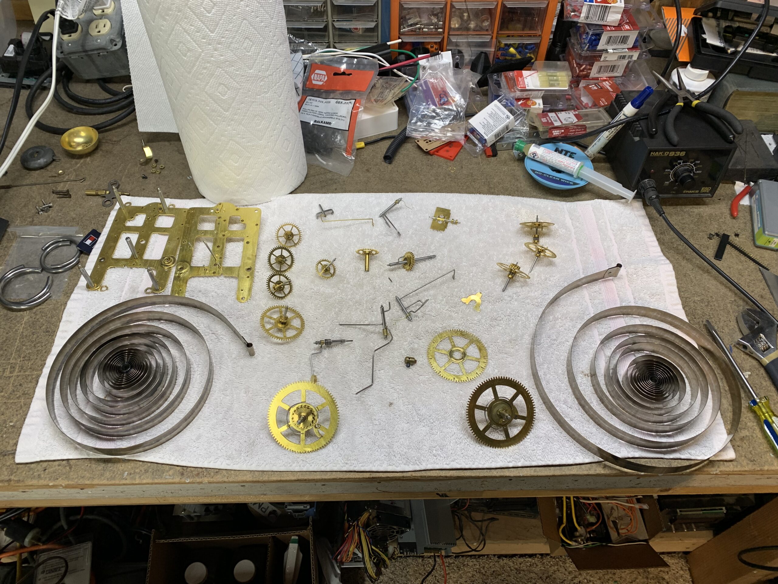
After I finished disassembling, cleaning, oiling, and putting everything back together, I was curious about how well this unit keeps time. Setting the time, and checking in to do manual readings, and trying to adjust the pendulum based on that is at best a pain. Instead, I decided to science it up.
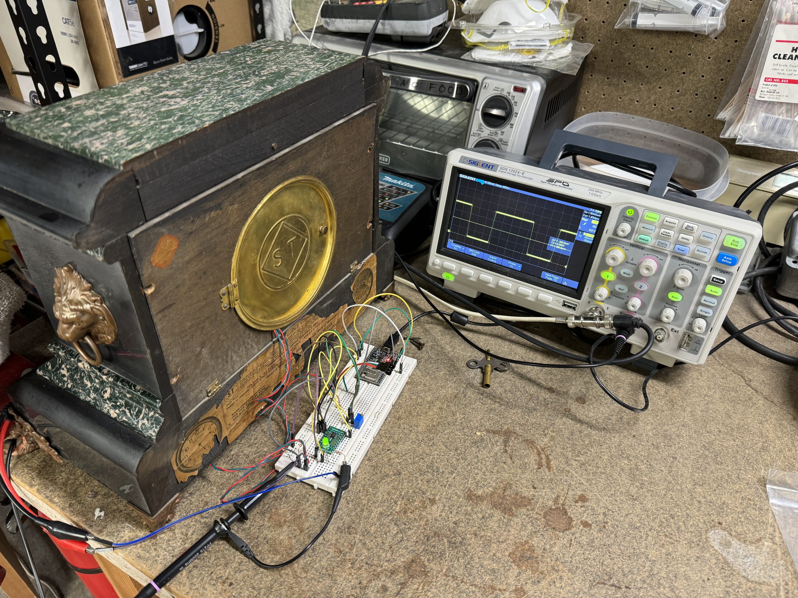
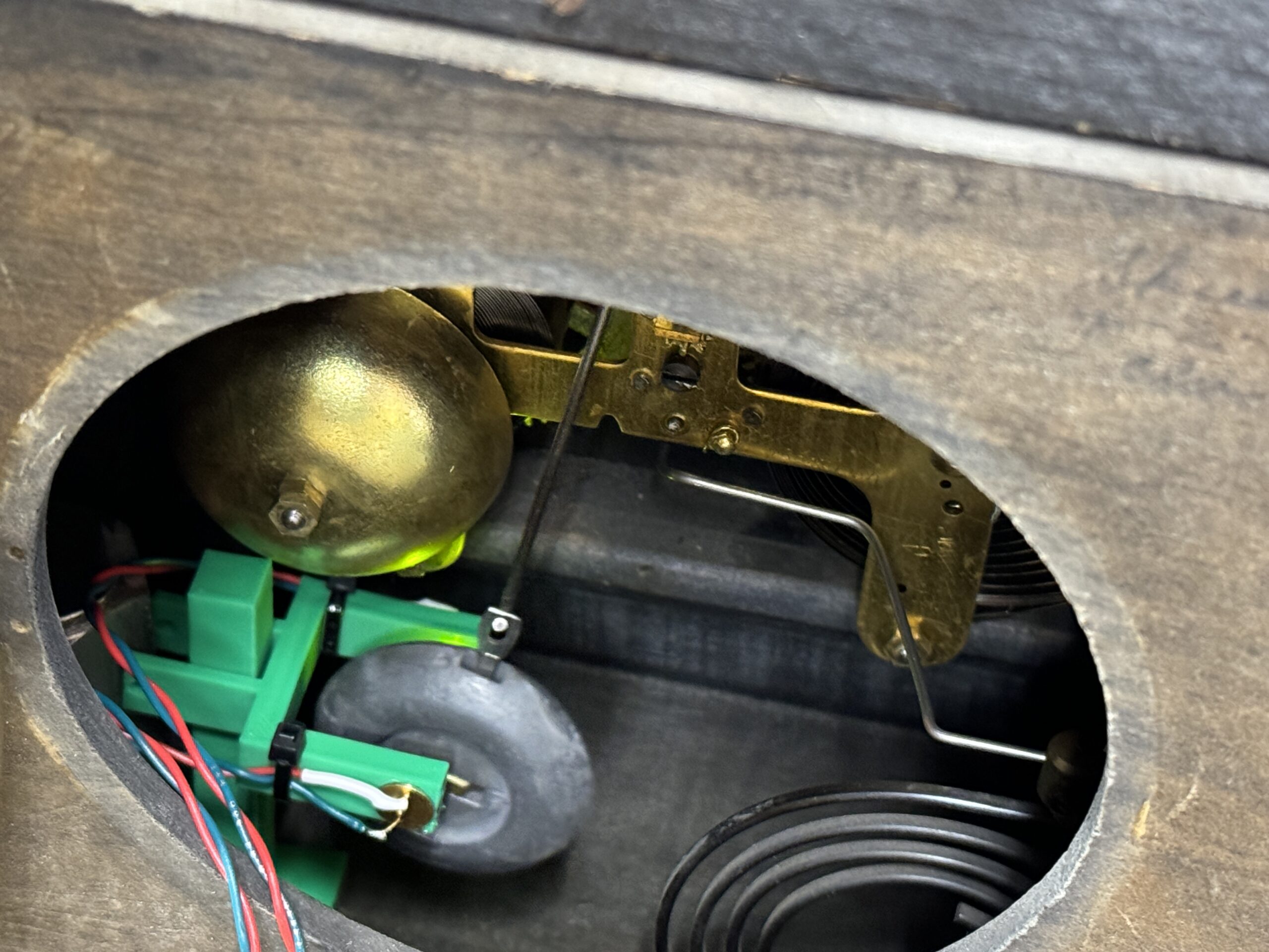
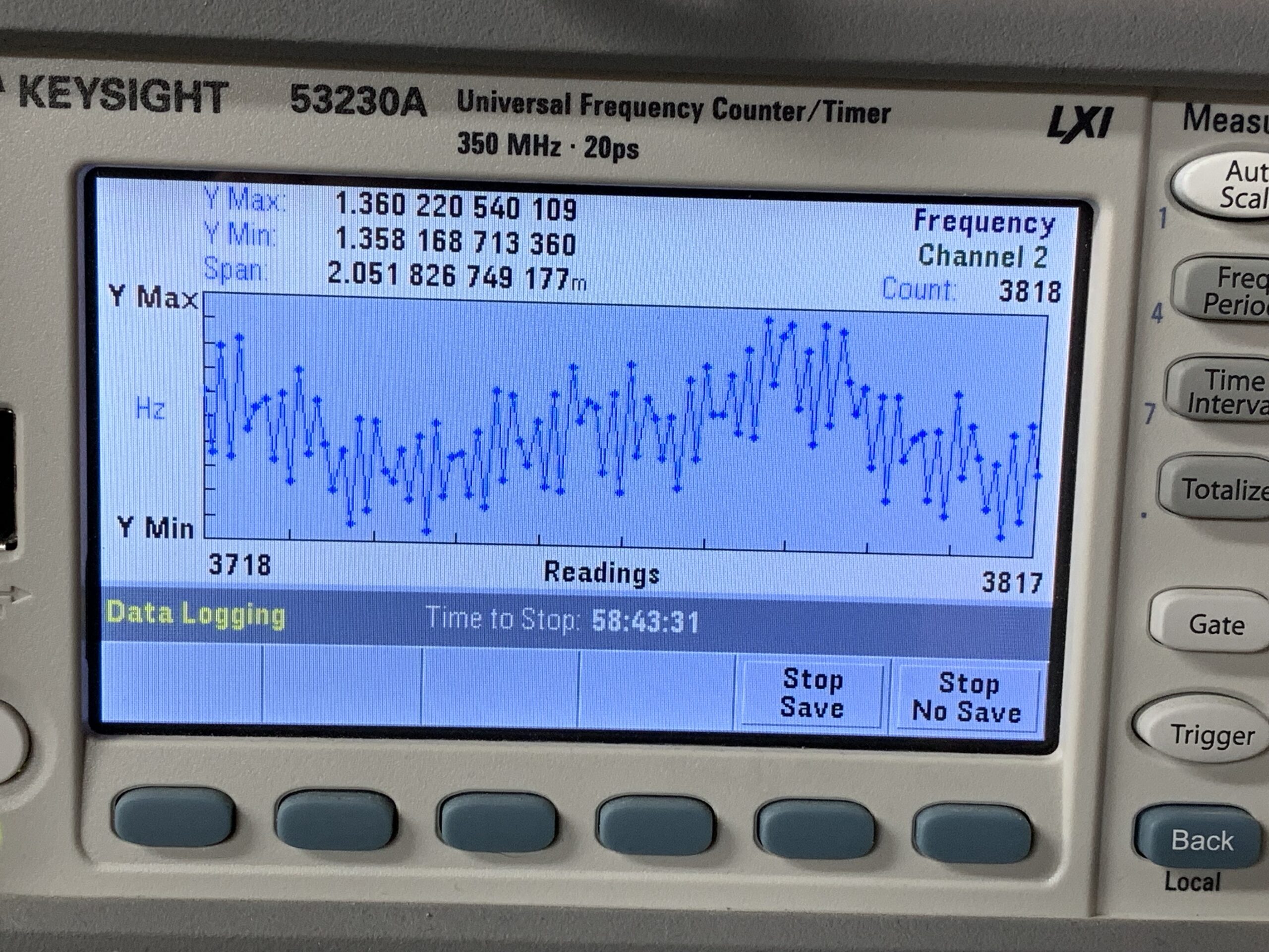
I quickly threw together a detector circuit with an LED, and a photodiode. Together with a little 3D printed ‘Y’ to hold the detector around the swinging pendulum, this allowed me to electronically and reliably measure the pendulum frequency. Doing the math based on the gears in the mechanism, I determined that 1.358035Hz is the frequency the pendulum needs to swing at to keep perfect time. I logged the pendulum frequency for 72Hrs, and then plugged the data into TimeLab to look at how the clock held time over the test.
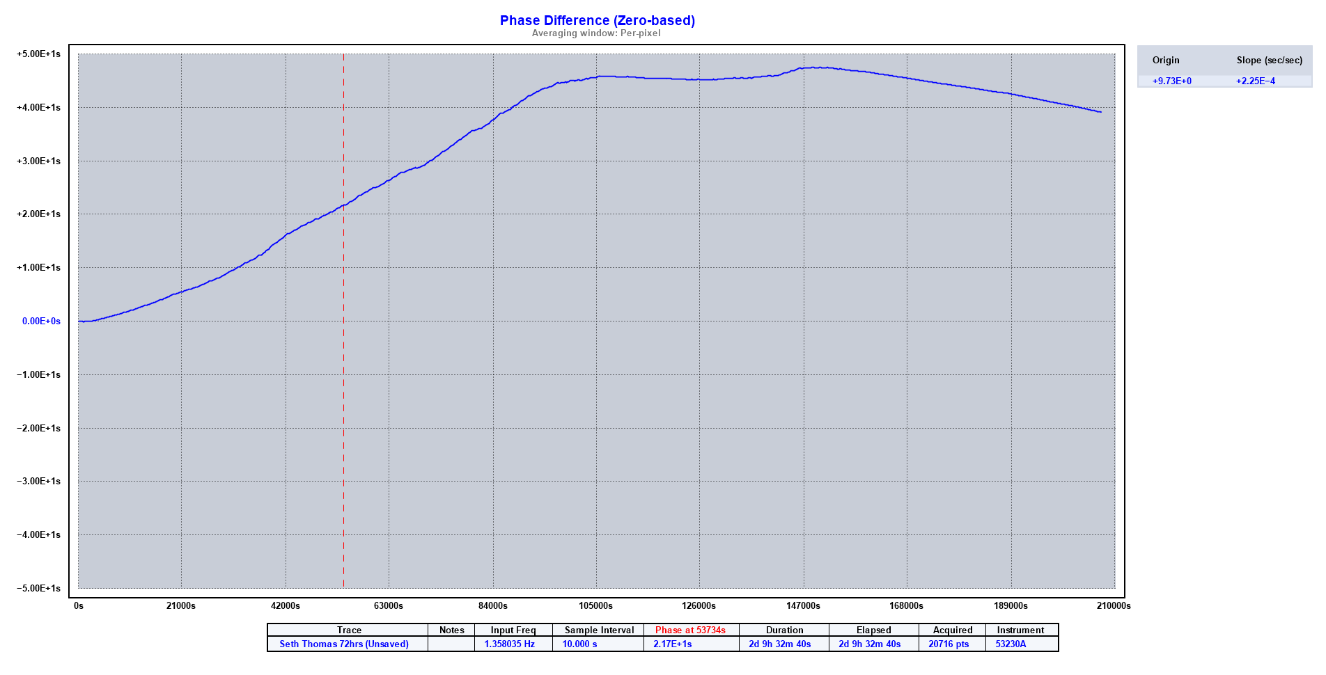
On this plot, we have our nominal ‘perfect’ frequency at the center of the vertical axis marked as `0.00E+0s`. This graph references the phase difference of the measured value as compared to the ideal frequency. Values above 0 represent the clock running fast, and values below represent the clock running slow.
So here we see that with the clock fully wound at the start, the clock is running fast, moving farther and farther ahead (by a few seconds) over the course of the first ~26 hours. After that, we hit a plateau where the clock is roughly running at a stable frequency, not gaining or losing time. The spring seems like it’s wound at just the perfect tension during this period. After that we see it start to lose time again as the spring unwinds further. This downward slope ends up bringing us closer to the initial setpoint again, but would continue past the setpoint as it continues to run slow.
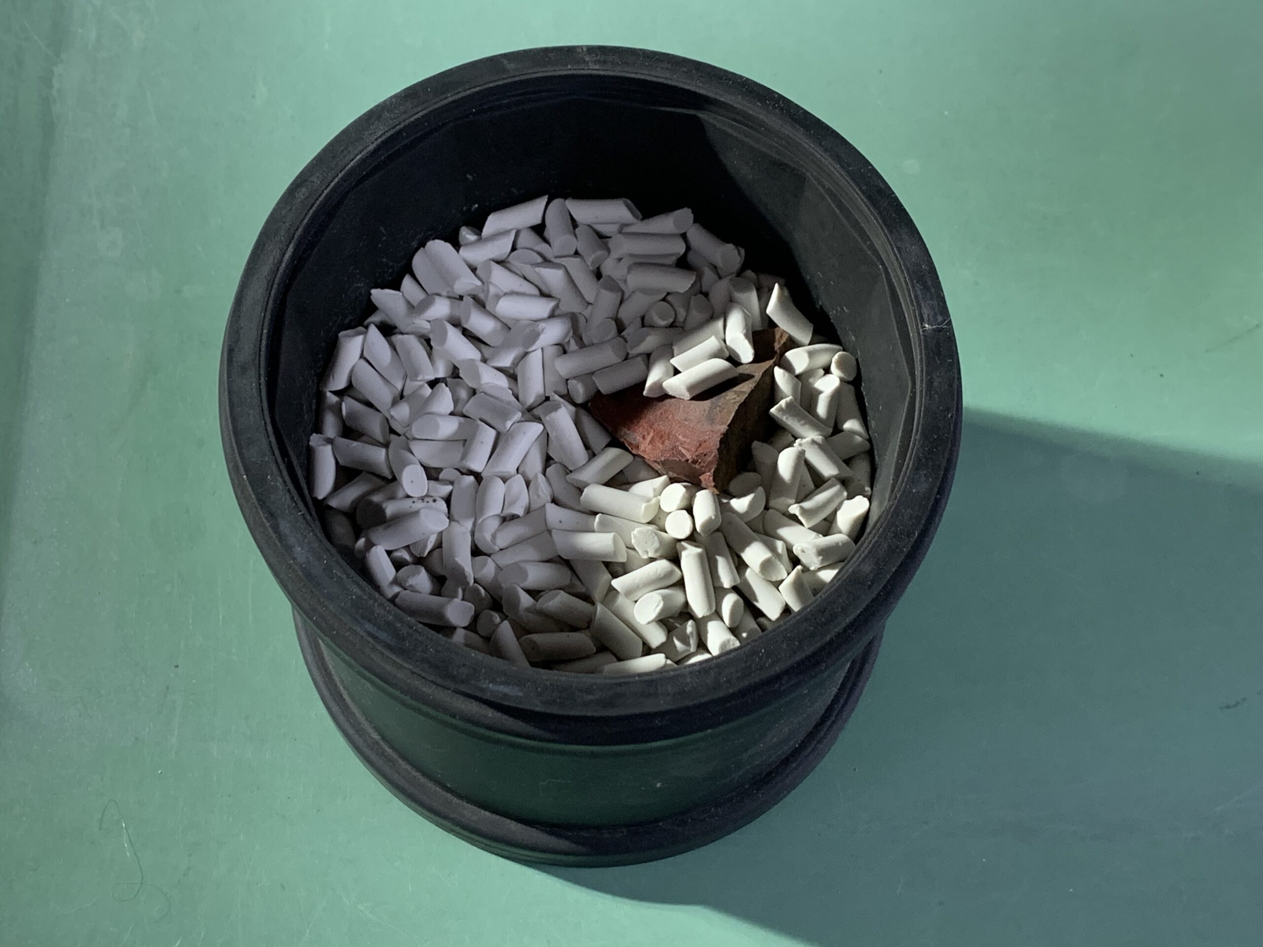
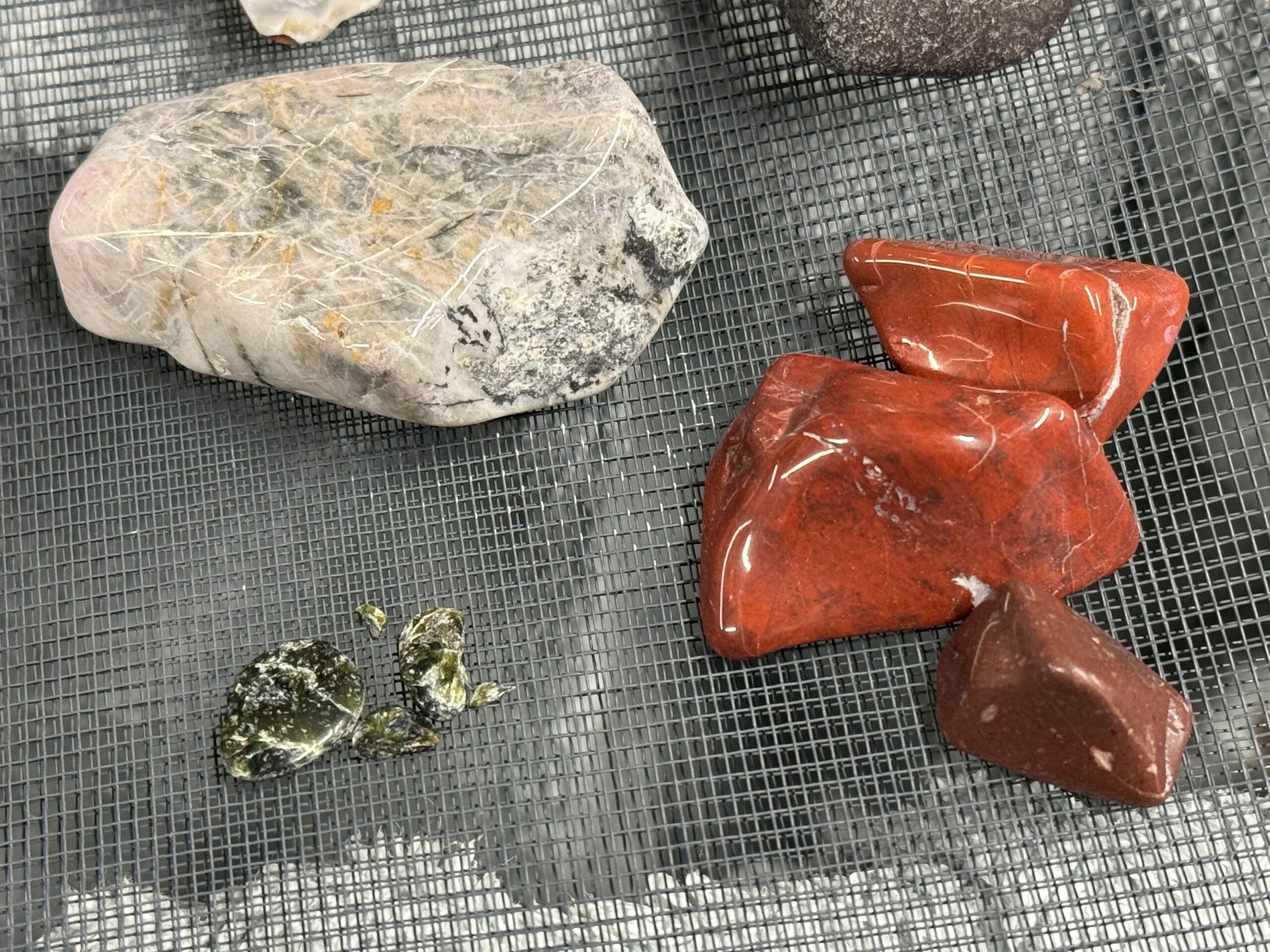
I recently came across some interesting looking assortment bags of rocks for tumbling from Dan Hurd Prospecting, and decided to pull out the old tumbler and give them a go.
The rocks arrive as rough chunks, and are loaded into the tumbler with some coarse grit, and some ceramic media.

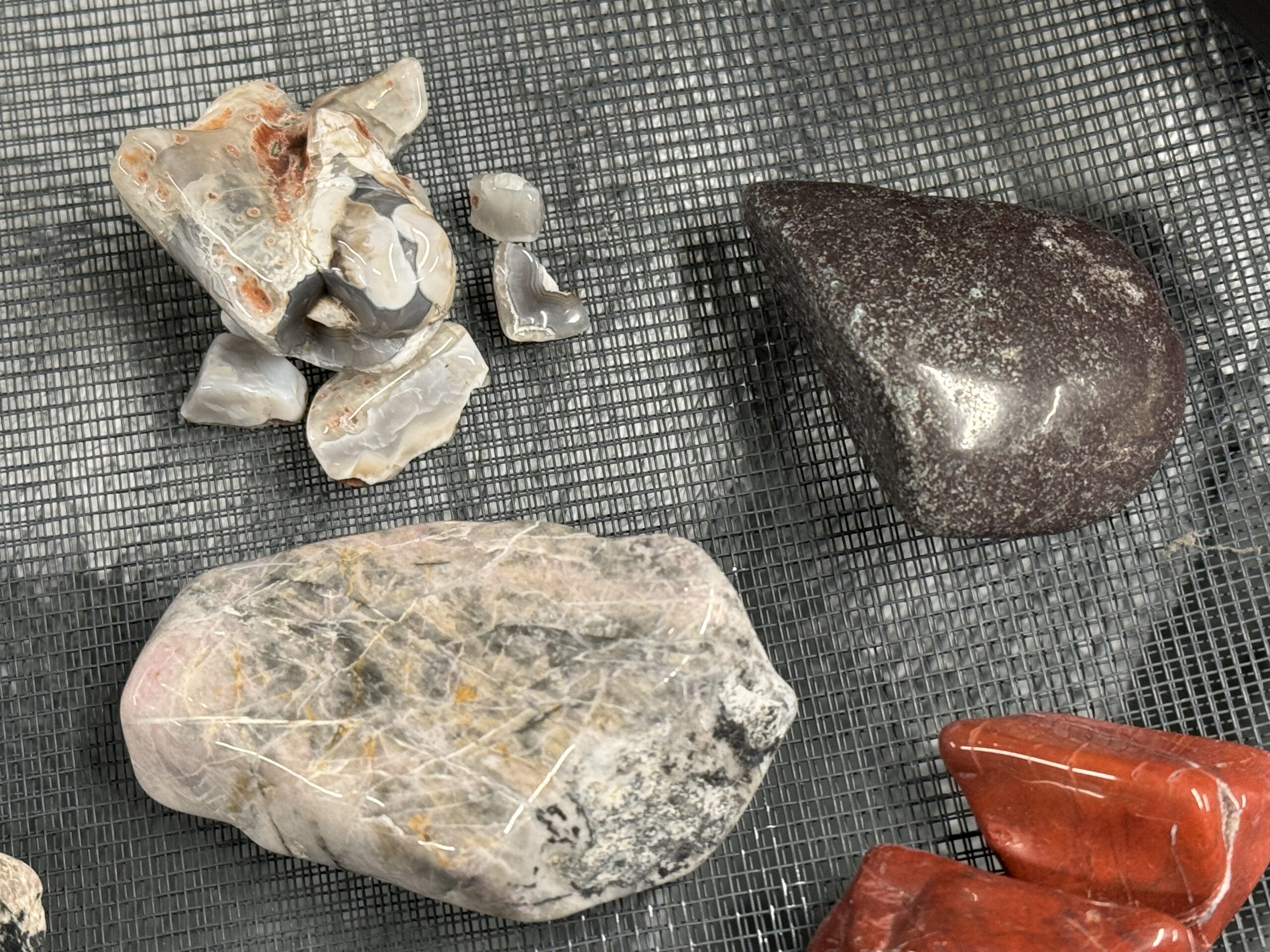
After the coarse and medium grits are completed they have the edges all rounded off, some of the stones have broken up into some smaller pieces, and they’re shiny while wet, though when dry they still have a matte finish.


They go back in for more rounds of tumbling, now with the fine and polishing grits, and come out shiny and finished. Some of the pieces broke up a little more, but overall I’m pretty happy with the results.


I was recently having a conversation with a colleague about doing some troubleshooting on a fiber optic network connection he was working on, and was looking for a way to verify light was actually making it down the fiber.
There are of course specialized tools that will measure this, and you can also get inexpensive ‘business cards’ with a coating that lights up visibly when you shine IR on them. However, even better is something you have with you all the time. Your smartphone!
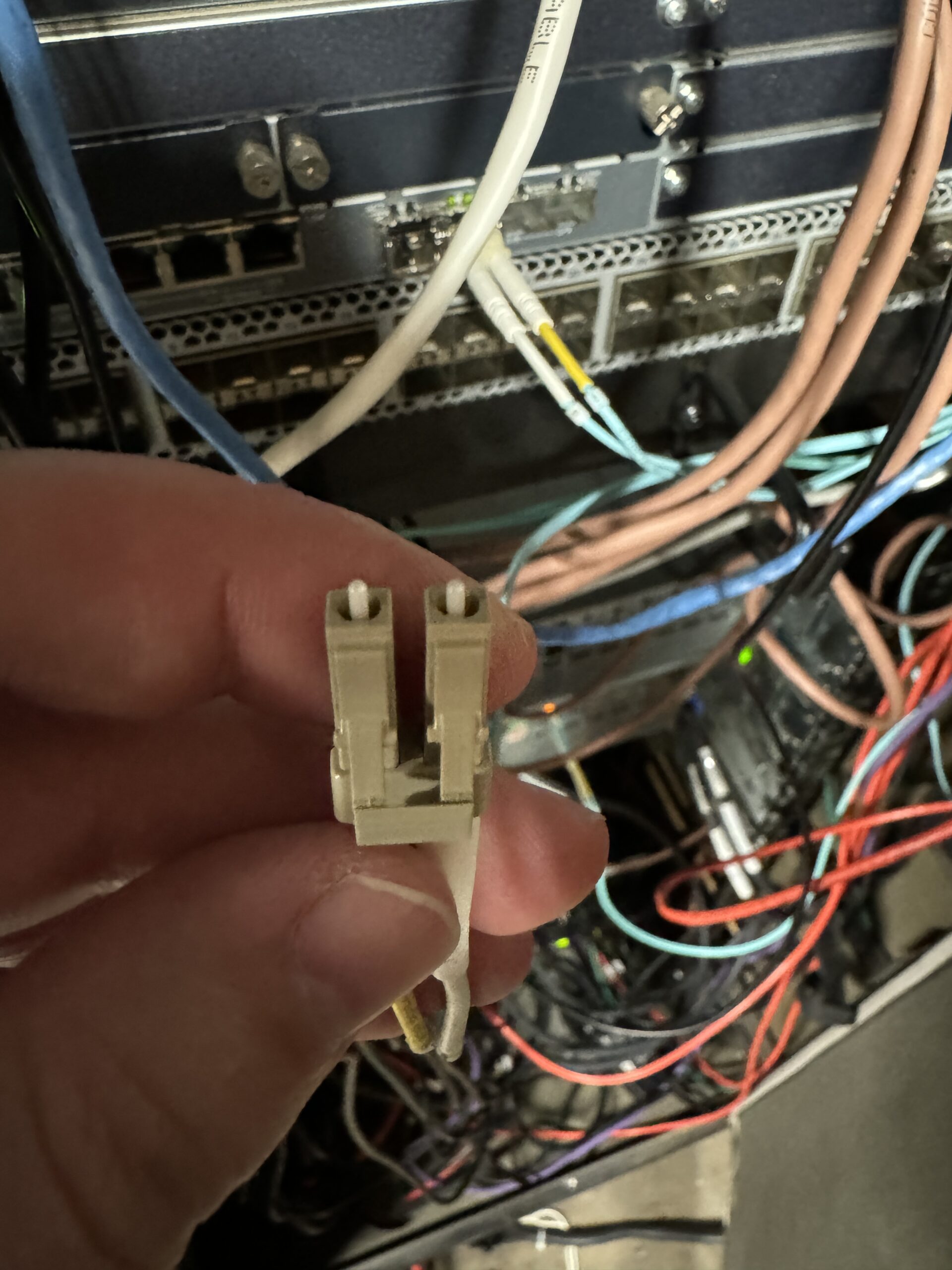
The camera in almost all smartphones is at least somewhat sensitive to IR light, so you can do a quick check using your phone. This trick also works for TV remotes if you’re not sure if the batteries are dead.
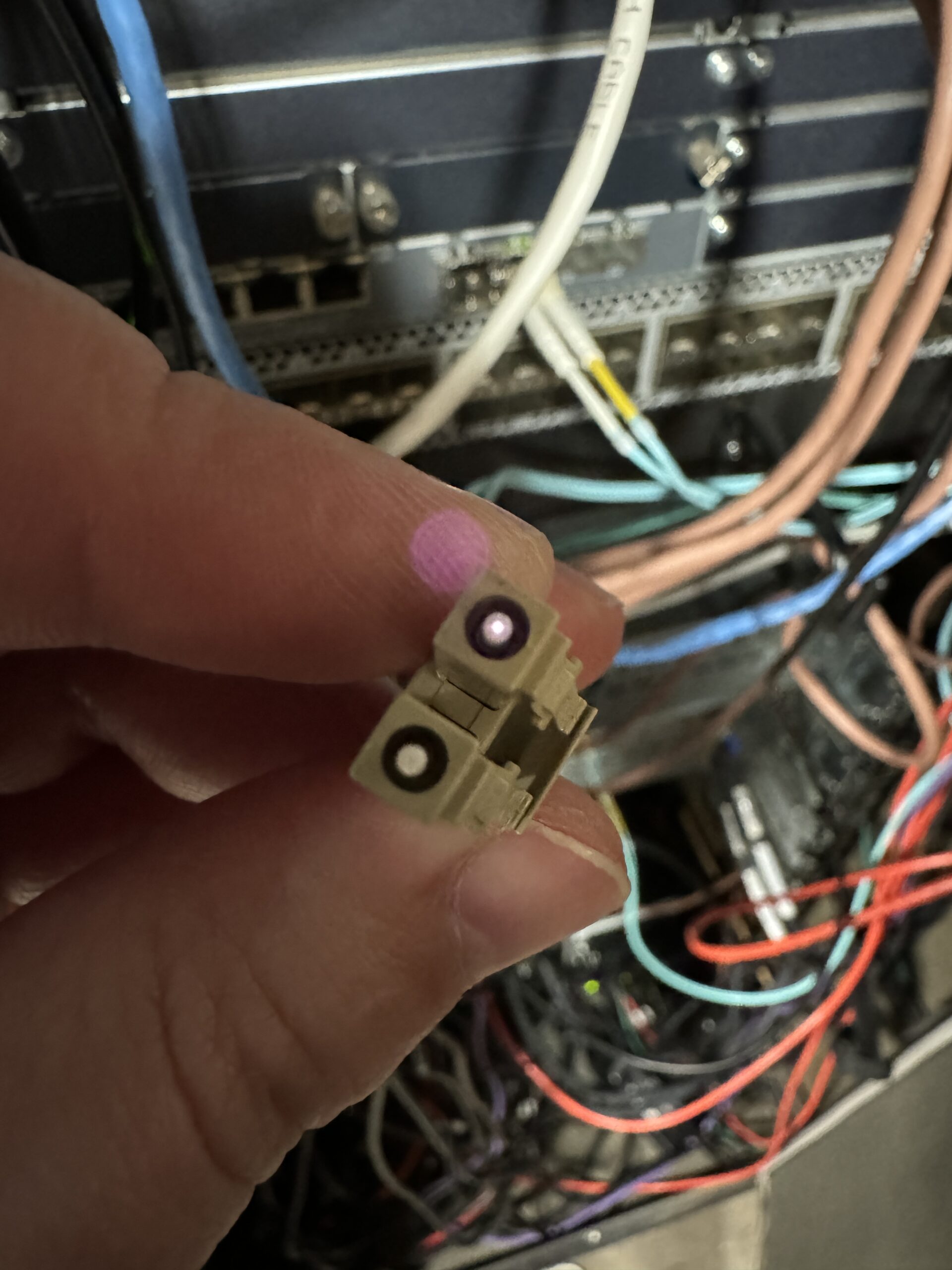
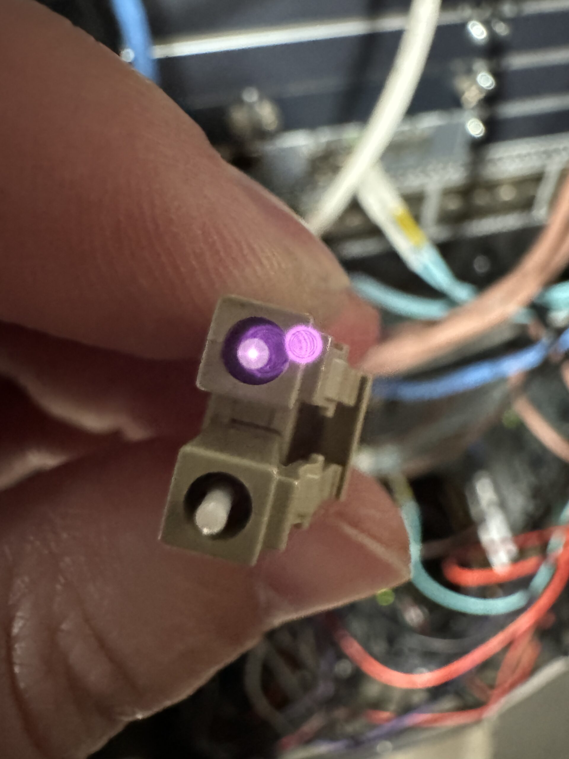
On an LC connector like this, you should expect to see light on one side, and the dark one is for the return signal from the optic you’re plugging it into.
Just be careful not to look at the laser with your remaining good eye!
Many portable air conditioners are known to be problematic, and often reviled, for using a single hose to vent hot air outside. The problem with which, is that the air that gets pumped outside has to be replaced in your home, and that air is just going to come in from outside.
This cycle of pumping out hot air, and that being replaced with more hot air from outside, makes them less effective at cooling spaces, and you waste electricity running them more.
They do make two-hose models, which solve this problem by using a second hose to bring in outside air to exchange over the radiator before pumping it out again, resulting in no outside air being brought into the house.
Unfortunately these two-hose models are the significant minority, and unfortunately the impacts/benefits are nebulous. When all you know is that they’re ‘better’ but not really any information on how much better, it’s hard to justify buying a more expensive model.
I’ve had a single hose model for a few years to cool my basement office/workshop space, and have left it run as designed until now, knowing that it’s ‘less efficient’ but not putting really much thought into it. However, the wildfire smoke recently made me rethink trying to retrofit my unit into a two-hose operation, and try to reduce the amount of outside air (and pollutants) being pulled into the house.
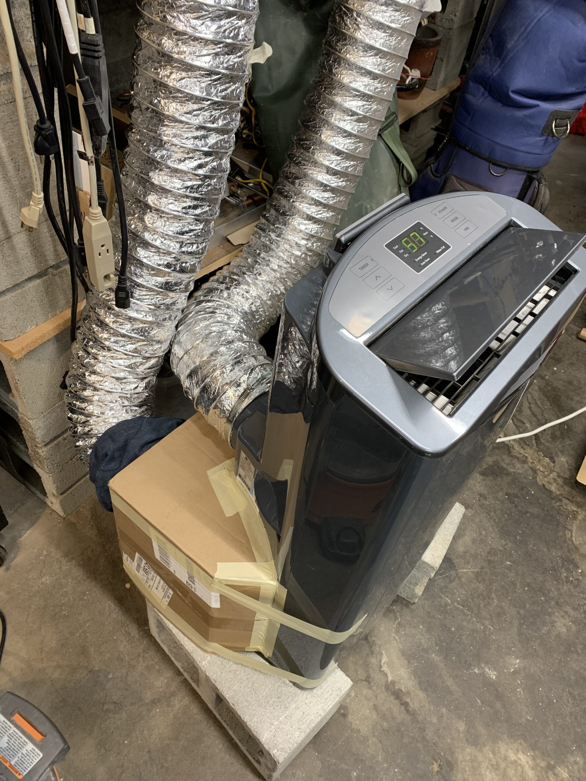
I cut and taped a cardboard box to enclose the intake portion of the radiator, and fed in some 6″ ducting from the hardware store, which matches the ducting for the exhaust, and fed both hoses out through the window.
First impressions are that subjectively it does feel like it does a better job of cooling. I don’t feel like I have to run it as hard, or turn the set temperature down as low to get the room to where I want it. However, subjective data is easily biased, and also isn’t great for convincing others.
Fortunately I have both indoor and outdoor air quality (particulate) sensors, and the data shows a remarkable change.
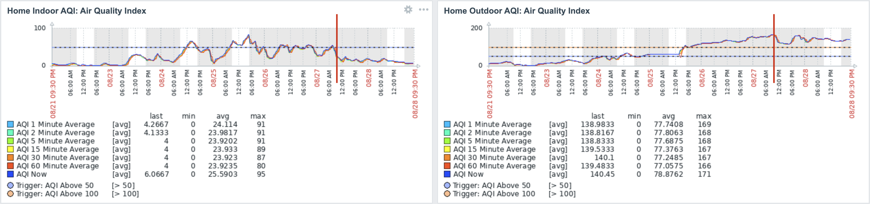
We are looking at a 7 day graph window, and we can see in the Indoor graph, that for a large portion of the earlier part of the week, I have been fighting to keep air quality inside the house at a reasonable level, using box fans with filters, and occasionally running the central furnace on fan mode to pull air through the furnace filter as well.
The marked red line is where I modified the air conditioner to two-hose operation. After which we see a very significant drop off and better air quality inside the house without having to run the central furnace fan/filter. Meanwhile air quality levels outside remain well above an AQI of 100, so the improvement in indoor quality is not due to an improvement outdoors.
To me, this is pretty clear evidence just how much air this portable air conditioner was causing the house to exchange with the outdoors, and how much of an impact it can have on the efficiency of cooling the house, as well as in situations like mine where there is wildfire smoke, the air quality within the house.